Elastic Distributed Calculation Engine
| Author | XAP Version | Last Updated | Reference | Download |
|---|---|---|---|---|
| Shay Hassidim | 12.0.1 | Feb 2017 | Example |
Overview
Financial services, Healthcare, Transportations, Fraud Detection, Payment systems, etc. produce reports constantly. Some of them produce reports where the data required for the report is generated over night via batch processing, and some other type of reports are produced instantly upon user request. This type of processing activity requires fast access to the raw data and the ability to utilize distributed resources available on the local environment or on the cloud.
The Elastic Calculation Engine example illustrates the following:
- Calculating Net present value (NPV) for large amounts of trades in real time using an In-Memory Data Grid.
- Intelligent Map-Reduce directing calculations into distributed nodes, lowering the network traffic and lowering the load on each calculation node.
- Simulating lazy data load in a batch mode optimizing database access in case of a cache miss.
- While the calculation is going on, dynamically scaling up and down the compute/data grid. This will increase the capacity of the compute/data grid and will allow it to utilize additional CPU resources to speed up the calculation time.
The Distributed Calculation Engine performs Net Present Value calculations where the Trades used for the calculation divided into several Books. These books could represent different types of Trades, different markets, different customers , etc.
Colocated vs. Remote Calculations
Calculations can be deployed colocated with the data or separately.
| Functionality | Colocated Calculations | Remote Calculations |
|---|---|---|
| Calculation impact on data grid node CPU utilization | Yes. Controlled. | No |
| Calculation impact on Data Grid node memory utilization | Yes. Controlled. | No |
| “Bad Calculation” may cause Data-Grid instability | Yes. Each node recovers independently | No |
| Data access overhead | Low | High. May be optimized via batch operations |
| Scaling flexibility | Data-Grid and Calculations scale in 1:1 ratio | Data-Grid and Calculations scales independently |
| Transactional | Yes | Yes |
| Persistency Support (write behind) | Yes | Yes |
| Hot deploy (refresh node code dynamically without downtime) | Yes | Yes |
| Calculation splitting support | Yes. Intelligent routing support. | Yes |
| Recommended with | Lightweight calculations. No IO | Heavyweight calculations. CPU / IO bound |
Colocated Calculations
The Calculating Flow
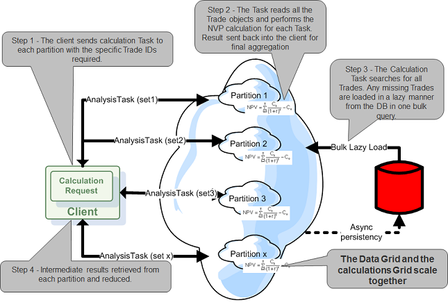
The Calculating Flow includes the following:
- A client, splitting a list of Trade IDs into multiple batches. Each Batch is sent into the calculation node (space partition) via a AnalysisTask that implements the Task Interface. Each calculation node stores a subset of the Trade data.
- The AnalysisTask is executed. Once completed, an intermediate result is sent back to the client. If the requested Trade cannot be found within the space, it is loaded from the database.
- The client aggregating the results retrieved from all the calculations nodes and reducing it to four numbers. These four numbers represent books.
When running the Elastic Calcualtion Engine on a single machine, scaling up and down will not affect the calculation time, but when running this on a grid with multiple machines, you will see better or worse calculation time when the grid scales up or down.
Intelligent Map-Reduce
The Elastic Calcualtion Engine uses the ExecutorBuilder. This allows executing multiple AnalysisTasks in a parallel manner where each Task includes a different Trade ID list to use for the calculation. Each List is sent to a relevant node where it is used to fetch the Trade data from the colocated space or to be loaded from the database.
The AnalysisTask
The AnalysisTask include the following:
executemethod - invoked on each partition. It returns a sum of all of the calculated NPV values for all the trades found within the partition divided by books. The demo assumes there are four books.getTradesFromDBmethod - used to load missing Trade objects from the database. Since this demo does not include a running live database the Trade data is generated via random data.calculateNPVmethod - called by the execute method to calculate the Net present value for the Trade.
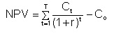
The Net Present Value (NPV) Calculation
The Net Present Value calculation calculates the NPV for 6 years. It is using the following code:
public void calculateNPV(double rate , Trade trade) {
    double disc = 1.0/(1.0+(double)(rate/100));
    CacheFlowData cf =  trade.getCacheFlowData();
    double NPV = (cf.getCacheFlowYear0() +
            disc*(cf.getCacheFlowYear1() +
            disc*(cf.getCacheFlowYear2() +
            disc*(cf.getCacheFlowYear3() +
            disc*(cf.getCacheFlowYear4() +
            disc*cf.getCacheFlowYear5())))));
    trade.setNPV(NPV);
}
The above can be described using the following formula:
The NPVResultsReducer
The NPVResultsReducer receives the NPV calculation for each book from each calculation node (partition) and reduces it into a list of NPV values for each book (four values).
The Trade
The Trade Space class stores the following items:
- id - The Trade ID.
- CacheFlowData - The cache flow data for Year 0 through Year 5.
Elasticity
The Elastic Processing Unit is used to deploy the data/compute grid and scale it dynamically. This allows you to increase the capacity of the data grid and leverage additional CPU resources for the calculation activity. With this demo, the user changes the capacity using a scale command that instructs the data/compute grid to increase its capacity (this in turn starts additional containers and re balances the data/compute grid) or decrease its capacity (by terminating containers and re balancing).
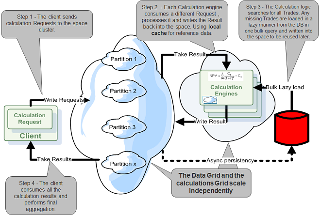
Remote Calculations
For long calculations that consume relatively large amount of CPU time, the recommended approach to implement distributed calculations is the Master-Worker Pattern. The approach suggested with the Master-Worker pattern should be used when the calculation time is relativity very long where the data access time can’t be considered as overhead.
Running the Demo
1. Download the ElasticCalculationEngine.zip and extract it into an empty folder. Move into the ElasticRiskAnalysisDemo folder and edit the setExampleEnv.bat to include correct values for the XAP_NIC_ADDRESS and the GS_HOME variables.
2. Start the XAP agent by running the following:
startAgent.bat
You will need a machine with at least 2GB free memory to run this demo.
3. Run the Elastic Data-Grid deploy script:
deployDataGrid.bat
This will deploy the data grid/compute grid and will later allow you to scale it. Whenever you would like to scale the data grid/compute grid just hit Enter. Running the deploy script again will initiate the scaling cycle again for the existing running data grid/compute grid.
4. Scale the Data-Grid using the scaleDataGrid script
scaleDataGrid.bat
This will allow you to scale it from 256MB , to 512MB , to 1024MB and back to 256MB.
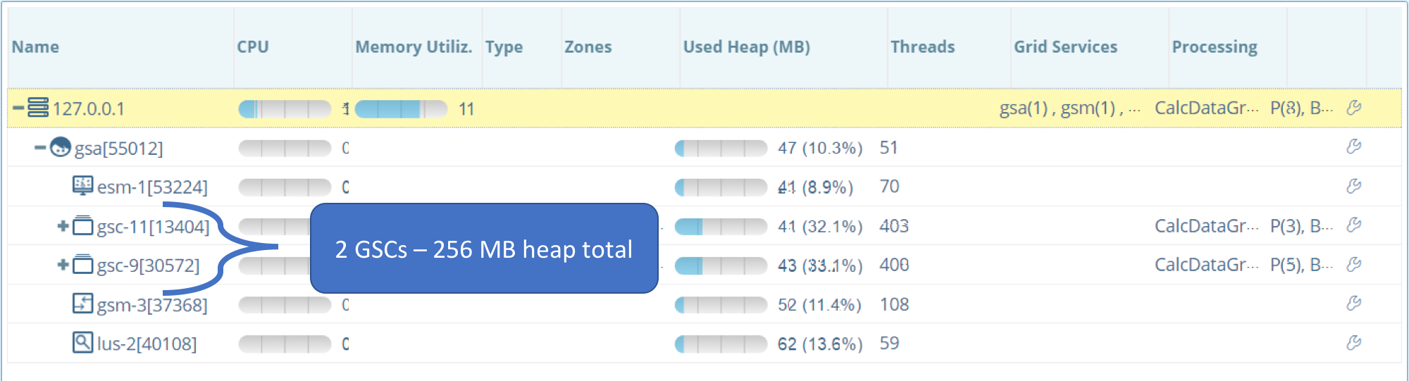
Using the Web Management Console you can see how the scaling takes effect:
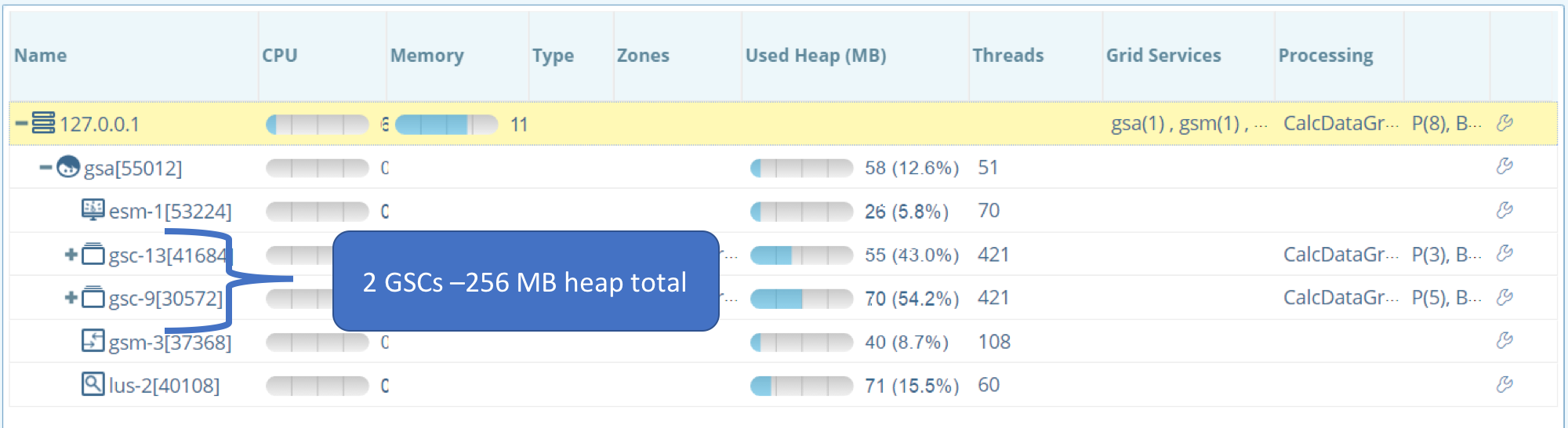
4.1 Initial State - 256 MB Capacity
4.2 Scale to 512MB
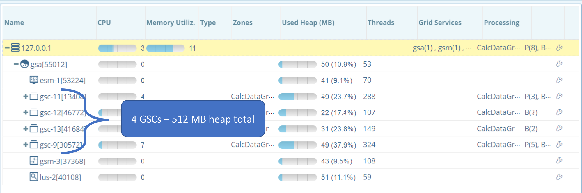
4.3 Scale to 1024MB
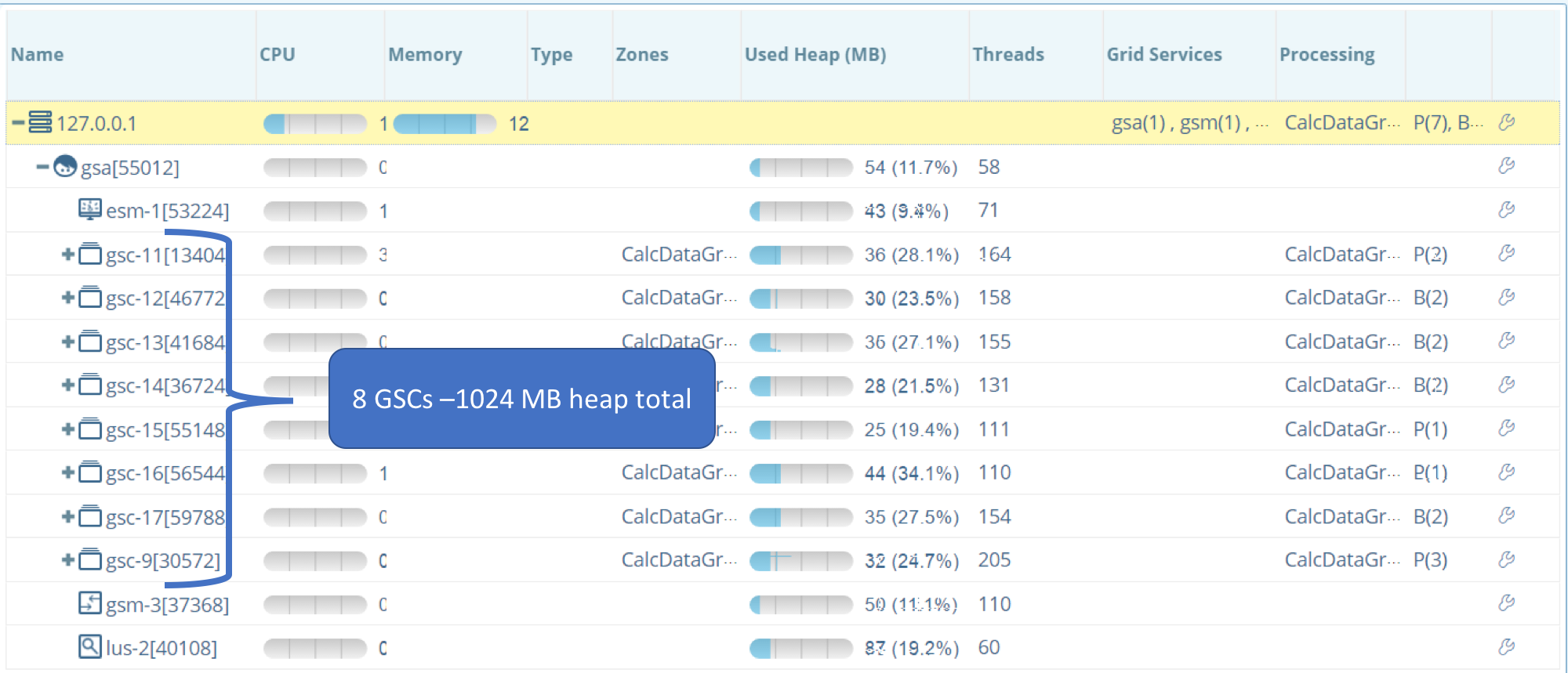
4.4 Scale back to 256MB
Colocated Calculations Demo
At any point you can run the calculation logic using the Colocated Tasks using runClientExecutor.bat
runClientExecutor.bat
Remote Calculations Demo
1. Deploy the Elastic Worker:
deployWorker.bat
This will deploy the Worker PU into the exiting Service Grid.
2. Run the client invoking the Remote calculations (this will be using the worker PU):
runClientMasterWorker.bat
The client will run the calculation repeatedly for 10,000 Trades where each cycle will use different rates (2%, 3%, 4%, 5%, 6%, 7%, 8%). To stop the client hit CTRL + C.
3. To scale the worker run the following:
ScaleWorker.bat
and follow the instructions. You can add or remove workers.
Running within eclipse
You may run the Calcualtion Engine within eclipse by using the StartCluster main class. It will start a clustered space. You can use this to debug the AnalysisTask when executed at the space side.
Expected Output
When scaling from 256 MB to 512 MB:
Thu Feb 23 15:52:31 EST 2017 Total GSCs:2 Total Heap[MB]:257
Thu Feb 23 15:52:32 EST 2017 Total GSCs:2 Total Heap[MB]:257
Thu Feb 23 15:52:33 EST 2017 Total GSCs:2 Total Heap[MB]:257
Thu Feb 23 15:52:34 EST 2017 Total GSCs:4 Total Heap[MB]:514
Hit Enter to scale Data Grid to 1024m
When scaling from 512 MB to 1024 MB:
Thu Feb 23 15:53:42 EST 2017 Total GSCs:4 Total Heap[MB]:514
Thu Feb 23 15:53:43 EST 2017 Total GSCs:4 Total Heap[MB]:514
Thu Feb 23 15:53:44 EST 2017 Total GSCs:4 Total Heap[MB]:514
Thu Feb 23 15:53:45 EST 2017 Total GSCs:4 Total Heap[MB]:514
Thu Feb 23 15:53:46 EST 2017 Total GSCs:8 Total Heap[MB]:1028
Hit Enter to scale Data Grid to 256m
When scaling from 1024 MB to 256 MB:
Thu Feb 23 15:55:30 EST 2017 Total GSCs:8 Total Heap[MB]:1028
..
Thu Feb 23 15:55:44 EST 2017 Total GSCs:7 Total Heap[MB]:899
...
Thu Feb 23 15:56:04 EST 2017 Total GSCs:6 Total Heap[MB]:771
...
Thu Feb 23 15:56:52 EST 2017 Total GSCs:3 Total Heap[MB]:385
...
Thu Feb 23 15:56:53 EST 2017 Total GSCs:2 Total Heap[MB]:257
We have 8 partitions
2017-02-23 16:36:39,578  INFO [Client] - Calculating Net present value for 10000 Trades ...
2017-02-23 16:36:39,703  INFO [Client] -
Time to calculate Net present value for 10000 Trades using 2.0 % rate:122 ms
2017-02-23 16:36:39,705  INFO [Client] - Book = Book0, NPV = 2237537745.8
2017-02-23 16:36:39,705  INFO [Client] - Book = Book3, NPV = 2238880805.7
2017-02-23 16:36:39,705  INFO [Client] - Book = Book1, NPV = 2237985432.4
2017-02-23 16:36:39,706  INFO [Client] - Book = Book2, NPV = 2238433119.1
2017-02-23 16:36:40,739  INFO [Client] -
Time to calculate Net present value for 10000 Trades using 3.0 % rate:33 ms
2017-02-23 16:36:40,739  INFO [Client] - Book = Book0, NPV = 4353811571.6
2017-02-23 16:36:40,740  INFO [Client] - Book = Book3, NPV = 4356424903.9
2017-02-23 16:36:40,741  INFO [Client] - Book = Book1, NPV = 4354682682.4
2017-02-23 16:36:40,742  INFO [Client] - Book = Book2, NPV = 4355553793.1
2017-02-23 16:36:41,773  INFO [Client] -
Time to calculate Net present value for 10000 Trades using 4.0 % rate:30 ms
2017-02-23 16:36:41,774  INFO [Client] - Book = Book0, NPV = 6354633987.8
2017-02-23 16:36:41,774  INFO [Client] - Book = Book3, NPV = 6358448293.9
2017-02-23 16:36:41,774  INFO [Client] - Book = Book1, NPV = 6355905423.1
2017-02-23 16:36:41,775  INFO [Client] - Book = Book2, NPV = 6357176858.5
2017-02-23 16:36:42,816  INFO [Client] -
Time to calculate Net present value for 10000 Trades using 5.0 % rate:40 ms
2017-02-23 16:36:42,816  INFO [Client] - Book = Book0, NPV = 8245475707.5
2017-02-23 16:36:42,817  INFO [Client] - Book = Book3, NPV = 8250424972.7
2017-02-23 16:36:42,817  INFO [Client] - Book = Book1, NPV = 8247125462.6
2017-02-23 16:36:42,817  INFO [Client] - Book = Book2, NPV = 8248775217.6
2017-02-23 16:36:43,863  INFO [Client] -
Time to calculate Net present value for 10000 Trades using 6.0 % rate:45 ms
2017-02-23 16:36:43,863  INFO [Client] - Book = Book0, NPV = 10031489134.5
2017-02-23 16:36:43,864  INFO [Client] - Book = Book3, NPV = 10037510436.5
2017-02-23 16:36:43,864  INFO [Client] - Book = Book1, NPV = 10033496235.2
2017-02-23 16:36:43,865  INFO [Client] - Book = Book2, NPV = 10035503335.8
2017-02-23 16:36:44,915  INFO [Client] -
Time to calculate Net present value for 10000 Trades using 7.0 % rate:50 ms
2017-02-23 16:36:44,916  INFO [Client] - Book = Book0, NPV = 11717530016.3
2017-02-23 16:36:44,916  INFO [Client] - Book = Book3, NPV = 11724563347.6
2017-02-23 16:36:44,916  INFO [Client] - Book = Book1, NPV = 11719874460.1
2017-02-23 16:36:44,916  INFO [Client] - Book = Book2, NPV = 11722218903.8
2017-02-23 16:36:45,980  INFO [Client] -
Time to calculate Net present value for 10000 Trades using 8.0 % rate:62 ms
2017-02-23 16:36:45,981  INFO [Client] - Book = Book0, NPV = 13308177424.2
2017-02-23 16:36:45,981  INFO [Client] - Book = Book3, NPV = 13316165525.9
2017-02-23 16:36:45,981  INFO [Client] - Book = Book1, NPV = 13310840124.8
2017-02-23 16:36:45,982  INFO [Client] - Book = Book2, NPV = 13313502825.3