Capacity Planning

Capacity planning is calculating the number of machines your application requires. This is one of the most important tasks you must complete before moving into production and making your application available to your customers/users. Typically, it should be done during the early stages of your project, in order to budget for the hardware and relevant software products your system will use. At a minimum, capacity planning involves estimating the number of CPUs and cores plus the memory each machine must have.

Another important deployment decision is to calculate the maximum number of data grid partitions the application requires. This deployment parameter determines the scalability of your application data grid. When the application is deployed, the number of data grid partitions remains constant, but their physical location, their activation mode (primary or backup), and hosting containers are dynamic.

The data grid instances can fail and relocate themselves to another machine automatically. They can relocate as a result of an SLA (Service Level Agreement) event (for example - CPU and memory utilization breach), or they can relocate based on manual intervention by an administrator. This data grid "mobility" is a critical capability that, beyond providing the application with the ability to scale dynamically and self-heal itself, can prevent over-provisioning and unnecessary overbudgeting of your hardware. You can start small, and grow as needed with your hardware utilization. Your capacity planning should take this fact into consideration.

To avoid over provisioning, you should start small, and expand your data grid capacity when needed. The maximum number of data grid partitions can be calculated, based on a simple estimation of the number of machines you have available, or based on the size and quantity of objects your application generates. This allows your application to scale while remaining resilient and robust.

This topic addresses the following capacity planning issues:

1. How do I calculate the footprint of objects when stored within the data grid?

2. What is the balance between the amount of active clients, machine cores, and the data grid process heap size?

3. How should the number of data grid partitions be calculated?

Object Footprint Within the Data Grid

The object footprint within the data grid is determined based on the following:

• The original object size - the number of object fields and their content size.

• The JVM type (32- or 64-bit) - a 64-bit JVM may consume more memory due to the pointer address size.

• The number of indexed fields - every indexed value means another copy of the value within the index list.

• The number of different indexed values - more different values means a different index list.

• The object UID size - the UID is a string-based field, and consumes about 35 characters. You may have the object UID based on your own unique ID.

Calculating the Object Footprint

The best way to determine the exact object footprint is via a simple test that allows you to perform some extrapolation when running the application in production.

To calculate the object footprint:

1. Start a single data grid instance.

2. Take a measurement of the free memory.

3. Write a sample number of objects to the data grid (~100,000 is a good number).

4. Measure the free memory again.

This test provides a very good understanding of the object footprint within the data grid. Bear in mind that if you have a backup running, you need double the amount of memory to accommodate your objects.

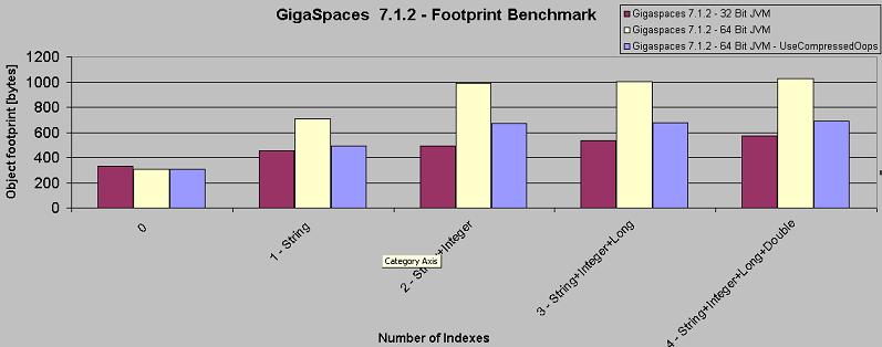
The following sample calculation of an object footprint uses a 32- and 64-Bit JVM with different amounts of indexes. The numbers below are for example only, and real results may vary based on the actual Object data and index values.

The test was set up as follows:

• Version XAP 7.1.2.

• All objects values are different.

• The Object has one String field, one Integer field, one Long field and one Double field.

• Footprint measured in Bytes.

• Basic Index type is used. An Extended Index type will have an additional footprint (20%) compared to a Basic Index type.

Indexes	Footprint 32-Bit JVM - Windows	Footprint 64-Bit JVM - Linux	Footprint 64-Bit JVM - UseCompressedOops - Linux
0	331	306	308
1 - String	456	705	493
2 - String+Integer	493	989	671
3 - String+Integer+Long	533	1002	680
4 - String+Integer+Long+Double	571	1026	691

Active Clients vs. Cores vs. Heap Size

The data grid kernel is a highly multi-threaded process, and therefore has a relatively large number of active threads handling incoming requests. These requests can come from remote clients or co-located clients, such as:

• Any remote call involves a thread on the data grid side that handles the request.

• A notification delivery may involve multiple threads sending events to registered clients.

• Any destructive operation (write, update, take) also triggers a replication event that is handled via a dedicated replication channel, which uses a dedicated thread to handle the replication request to the backup data grid instance.

• There is periodic background activity, used to monitor the relevant components that are using its own dedicated threads within the data grid kernel.

A co-located client does not go through the network layer, and interacts with the data grid kernel very fast. This means that the machine CPU core that has been assigned to deal with this thread activity is very busy, and does not wait for the operating system to handle IO operations. Taking this fact into consideration means we can have less concurrent clients served by the same core when compared to remote client activity.

The number of active threads and machine cores is an important consideration when calculating the maximum heap size to be allocated for the JVM running the GSC. You should keep memory in reserve for the JVM garbage collection activity, to deal with cleaning allocated resources and reclaiming unused memory. A large heap size means a potentially large number of temporary objects that can generate work for the garbage collection activity. You should have a reasonable balance between the number of cores the machine is running, the number of GSCs/data grids that are running, and the number of active clients/threads accessing the data grid.

A machine running 4 quad-core cores with fast CPUs (3GHz clock) can handle 20-30 concurrent collocated clients and 100-150 concurrent remote clients without any special delay. This JVM configuration should have at least a 2-3GB heap size to handle the data and additional resources that utilize the memory. With the above, we assume the application business logic is very simple and does not have any IO operations, and the data grid persistency mode is asynchronous.

Calculating the Number of Data Grid Partitions

Calculating the number of data grid partitions required by an application is essentially on the maximum number of machines available. You should have a dedicated machine per data grid instance hosted within a dedicated Grid Service Container (GSC).

The initial required number of GSCs per machine is calculated based on the machine's physical RAM, and the amount of heap memory you want to allocate for the JVM running the GSC. In many cases, the heap size is determined based on the operating system: for a 32-bit OS, you can allocate a 2GB maximum heap size, and for a 64-bit OS, you need 6-10GB maximum heap size (the JVM -Xmx argument). For performance optimization, you should have the initial heap size the same as the maximum size. The sections below demonstrate capacity planning using a simple, real-life example.

Here are a few basic formulas you can use:

Amount of GSCs per Machine = Amount of Total Machine Cores/2

Total Amount of GSC = Amount of GSCs per Machine X Initial amount of Machines

GSC max heap Size = min (6, (Machine RAM Size * 0.8) / Amount of GSCs per Machine))

Amount of Data-Grid Partitions = Total Amount of GSC X Scaling Growth Rate / 2

Where:

• Number of Total Machine Cores - total number of cores the machine is running. For a quad-core with 2 CPUs (Duo) machine this value is 8.

• Number of Data Grid Partitions - number of data grid partitions you need to set when deploying.

• GSC max heap Size - JVM Xmx value

• Number of GSCs per machine - number of GSCs you run per machine. This is a GSA parameter.

• Total amount of data in memory - number that should be estimated based on the object footprint you are storing within the space.

• Scaling Growth Rate - expansion ratio, usually between 2-10. This value determines how much to expand the data grid capacity without downtime.

• Initial number of machines - initial available machines to have when deploying the data grid.

• Machine RAM Size - amount of physical RAM a machine has.

• Total number of GSCs - total number of GSCs that are initially running when deploying the data grid.

Example 1 - Basic Capacity Planning

In this example, there are initially 2 machines used to run the data grid application. 10 machines may be allocated for the project within the next 12 months. Each machine has 32GB of RAM with 4 quad-core CPUs. This provides a total of 64GB of RAM. Later, when all 10 machines are available, there will be a potential 320GB of total memory. The memory is used both by the primary data grid and the backup data grid instances (exact replica of the primary machines).

The machines are running a Linux 64-bit operating system. Allocating 6GB per JVM as the maximum heap size for the GSC results in 5 GSCs per machine; 10 GSCs initially across 2 machines. When all of the 10 machines are in use, there will be 50 GSCs.

When a maximum of 40 GSCs are hosting the data grid, it is a good idea to have half of them (20 GSCs) running primary data grid instances and the other half running backup instances. Use this number to define the number of partitions the data grid is deployed with. Each machine will start 4 GSCs, which will join the GigaSpaces grid and allow the administrator to manually or automatically expand the capacity of the data grid during runtime.

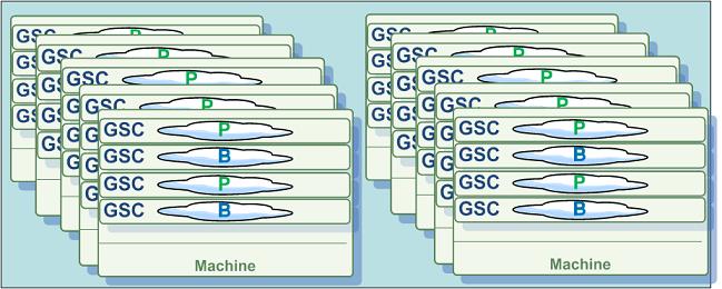
Figure 1: 10-Machine Topology. - 1 data grid Instance per GSC, total 320GB RAM

This rebalancing of the data grid instances can be done via the UI, or via a simple program using the Admin API.

Being able to determine the number of data grid partitions prior to the application deployment allows you to have exact knowledge of how your routing field values should be distributed, and how your data will be partitioned across the different JVMs that will be hosting your data in memory.

Example 2 - Capacity Planning when Running on the Cloud

In a cloud environment, you have access to essentially unlimited resources. You can spin up new virtual machines and have practically unlimited amounts of memory and CPU power. In this type of environment, calculating the maximum number of data grid partitions is not based on the maximum number of machines you might have allocated for your project because theoretically, you can have an unlimited number of machines started on the cloud to host your data grid. Still, you must have some value for the maximum number of data grid partitions when deploying your application. In this case, calculate the number of data grid partitions based on the amount of memory your application might generate and store within the data grid.

For example, if you have an application using 3 types of classes to store its data within the data grid:

• Class A - object average size is 1KB

• Class B - object average size is 10KB

• Class C - object average size is 100KB

The application needs to generate 1 million objects for each type of class during its life cycle:

• Class A - total memory needed = 1KB X 1M = 1GB

• Class B - total memory needed = 10KB X 1M = 10GB

• Class C - total memory needed = 100KB X 1M = 100GB

The total memory required to store the application data in memory = 111GB

When using machines with 32GB of RAM, 4 machines are needed to run enough primary data grid instances to store 111GB of data in memory, and another 4 machines are needed for the backup data grid instances. For a 64-bit operating system, the numbers are 5 GSCs, each having a 6GB maximum heap size for a total of 40 GSCs (5 X 4 X 2). This allows us to expand the data grid to run across 160 machines (one GSC per machine). This means 160 X 10GB as the heap size = 1.6TB of data grid memory capacity to host the data grid objects. This is a huge amount of capacity for the data grid, and actually 10 times larger than the estimated size. It provides a lot of room for error in case our initial memory utilization was wrong.

Used Memory Utility

Checking the used memory on all primary instances can be done using the following (we assume we have one GSC per primary instance):

GigaSpace gigaSpace = new GigaSpaceConfigurer(new UrlSpaceConfigurer(spaceURL)).gigaSpace();
Future<Long> taskresult = gigaSpace.execute(new FreeMemoryTask());
long usedMem = taskresult.get();
System.out.println("Used Mem[MB] " + (double)usedMem/(1024*1024));

The FreeMemoryTask implementation:

import java.util.Iterator;
import java.util.List;

import org.openspaces.core.executor.DistributedTask;

import com.gigaspaces.annotation.pojo.SpaceRouting;
import com.gigaspaces.async.AsyncResult;

public class FreeMemoryTask implements DistributedTask<Long, Long>{

    Integer routing;
    public Long execute() throws Exception {
        
        Runtime rt = Runtime.getRuntime();
        System.out.println("Calling GC...");
        rt.gc();
        Thread.sleep(5000);
        System.out.println("Done GC..." + 
                " Used memory " + (rt.totalMemory() - rt.freeMemory() )+
                " Free Memory " + rt.freeMemory() + 
                " MaxMemory " + rt.maxMemory() + 
                " Committed memory "+ rt.totalMemory());
        
        return (rt.totalMemory() - rt.freeMemory() );
    }

    @Override
    public Long reduce(List<AsyncResult<Long>> _usedMemList) throws Exception {
        
        long totalUsed =0;
        Iterator<AsyncResult<Long>> usedMemList = _usedMemList.iterator();
        while (usedMemList.hasNext())
        {
            totalUsed  = totalUsed + usedMemList.next().getResult();
        }
        return totalUsed ;
    }

    @SpaceRouting
    public Integer getRouting() {
        return routing;
    }

    public void setRouting(Integer routing) {
        this.routing = routing;
    }
}